After having analyzed the constraints with Collision analysis, the next step is to perform ground grading. This process involves modifying the terrain to align with the set criteria.

To start this calculation, click on the Grade button. You may choose to work with specific frames or with the entire PV area that was affected. The example below shows how to work with the entire PV area. Frames that are already adhering to the allowed ranges will be unaffected.

To initialize the process,  press Space or Enter. The process should take a couple of moments.

PVcase makes a copy of the existing topography in our PV area and any changes will be made using the copy rather than the original. The copy can be found in the PVcase Proposed Grade layer. However, only a small portion of the points are displayed.

This ensures no unwanted changes are made to the original topography, and we may later swap between the original and proposed grade to compare the terrain.
Once the grading is completed, none of the frames should be marked as affected by the Collision analysis.
You can also define if and in which case the grading is performed not only under, but also between the frames.

If you would like grading between frames, check the checkbox and enter the pitch up to which space between frames should be graded. In the example below, grading will only be performed (orange hatch) between frames where the pitch is lower than the set 13m:

To inspect how the piling and clearing was affected by the grading, go to the Collision analysis section and click on Show details. Now, if you zoom in, you’ll see that all values are all within the range we specified.

You can go to the Heatmap tab and toggle between the original topography and the proposed one. Switch to the Existing topography, which generally does not take long.

You are now presented with the piling lengths and clearance values that would have been given prior to the grading. If you toggle back to the Proposed grade, you will see that the values will be adjusted back to the values that are within our specified range.

Front view 

Another way to illustrate how the changes affected the piling and terrain would be to perform a Front-section view:

1. Click the drop-down menu next to the Cross-section button and select Front view.
2. When prompted, select the PV area boundary line.
3. Press Space or Enter to confirm.
4. Draw the Front-view line.
5. Place the drawing off to the side by clicking your target location.

The front-view will update automatically.

To see how the proposed and original topography compares, zoom into a front view cut and see a black line indicating original topography and yellow indicating proposed terrain.

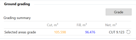
You can have a look at the Area grade section, where it is specified how much terrain had to be cut, filled and what is the net sum of the material being filled and removed.

You can also reset any proposed grading actions here:

Optimizing grading volumes

With the initial grading performed and examined, you may also try to reduce the amount of ground grading that is necessary to achieve the desired results (without modifying your constraints).
You can do this by setting a different reference height or using the Optimized mode (Frame and park settings, Height and optimization) before grading.

Before starting, it is highly advised to take screenshots or export the bill of materials. This is to retain the conditions with which we got the initial ground grading results.

Then reset all the grading actions from the initial grading. 

The previous grading resulted in more fill than cut. Your goal might be to decrease your net value by increasing the cut and decreasing the fill volume. You can do that by lowering our frames:

1. Go to Frame & Park settings
2. Click on Height and optimization
3. Decrease the reference frame clearance by 0.02 m (from 0.9 to 0.88)
4. Click OK to finalize
5. Select the PV area boundary line
6. Click Adapt to positions

All the frames in the area will now be lowered by 2 cm.

You can perform ground grading again, leaving the same clearance and/or piling length range as before. Repeat the steps by clicking on the Grade button and selecting the PV area boundary line and finalizing by pressing space or enter on the keyboard.

Once you are done with the grading, we open the screenshot or the previously generated Bill of materials spreadsheet file and compare the results.
As you can see, the second iteration yields a lower net value, thus optimizing the results. You may repeat this process as many times as necessary to get the most effective solution.

Instead of changing the reference clearance in Standard mode, you can also use the Optimized mode and adapt the range as desired for further iterations.

Grading heatmap
In the Grading heatmap tab, you can:

• Toggle between the existing and proposed terrain
• Export the existing or proposed terrain in CSV or LandXML format
• Compare the existing and proposed terrain with a heatmap or spot levels

The option to toggle between the Existing and the Proposed terrain allows you to choose the surface you want to work with. 

It also helps to visualize the changes in pile and clearance height before and after grading.

Surface comparison

After performing Ground grading, you can easily compare the existing and proposed grade surfaces using the heatmap in Surface comparison. There are two options to illustrate the grading intensity on the project area:

• The Heatmap colors affected segments of the terrain with a corresponding color
• Spot levels place text denoting the elevation difference in a specific spot on the drawing

Heatmap

Start by defining the values in the Surface comparison table.

• Starting value is the smallest value that will be represented in the heatmap

• Table range count defines the granularity of the heatmap (number of steps in either direction)

• Step size is the increment in which the values progress

Begin by defining your Starting value. In this example, it’s left at 0.05 m. It is generally best practice to have a Table range value of at least 5 — this allows for a better sense of granularity on the heatmap. Set the Step size to 0.1 m. Once we have the variables defined, click on Fill table and the table (right side of the window) will be populated.

The red color indicates the areas that are subject to material removal, while purple indicates areas where material needs to be added. You can customize the colors by clicking on them and choosing an option that suits your needs.
To see the heatmap switch the toggle On and Off — it takes a few seconds to appear.

Now you can see the surface heatmap, which illustrates which areas are subject to which type of grading procedure and at what intensity.

Spot levels

With Spot levels, you can define the density of the text element placement. This does not impact the accuracy of the grading procedure, but, rather, how many points are placed on the drawing to illustrate the calculations. The resulting elevations are colored based on the Surface comparison table. Use the toggle to switch the Spot levels on, as shown below:

If you export the Bill of material while the Spot levels option is on, the information is included in the spreadsheet:

Export to CAD

Finally, you can also add a legend with the surface comparison table colors and range values into the drawing:

1. Click on Export to CAD
2. Left-click on the drawing where you want to place the table

This is an accessible way to showcase the range of values and colors used for presentation purposes.